Wisdom Page: Kd measurement, fitting, calculation, and simulation

This wisdom page covers Kd measurements and calculations in direct measurement mode (the type of data that would be collected by fluorescence or NMR, for example).  Similar considerations apply for data collected in the derivative mode (ITC data), not discussed here.  I only treat single site binding here; this will cover 98% of the applications we will encounter in the Chazin lab.  Again, for multiple site binding the considerations are similar but (obviously) somewhat more complex.

Deriving and simulating the equations governing the behaviour of protein/ligand interactions can provide a significant base for understanding the limits of this measurement, including optimal concentration ranges for measuring certain ranges of Kd.  Critically, these simulations can provide an absolute floor or ceiling on the amount of error that can be expected in a given calculation. 

To begin at the beginning:

If protein P binds ligand A, then an equilibrium is formed:

P + A < -- > PA

Where P and A are free protein; PA is the ligand-bound-protein.

There is a ratio between the free species and the bound species. 

At a given set of conditions, this ratio is fixed:

Sometimes [P] is called [Pfree], and likewise [A] = [Afree]. Substituting, we get:

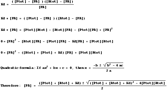
Now remember that the total amount of protein is divided into two "camps," free protein and ligand-bound-protein. Likewise for the total amount of ligand:

[Ptotal] = [Pfree] + [PA] which can be rewritten as [Pfree] = [Ptotal] - [PA]

[Atotal] = [Afree] + [PA] which can be rewritten as [Afree] = [Atotal] - [PA]

Therefore:

A little algebra as follows:

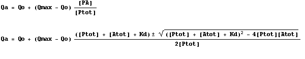
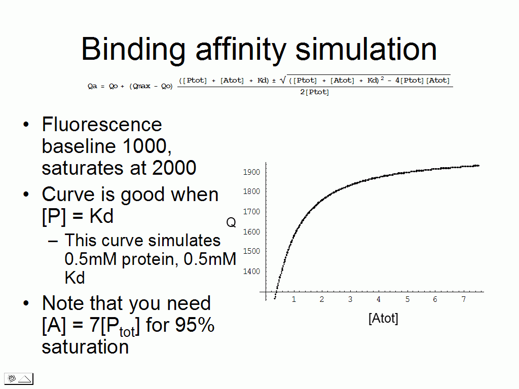
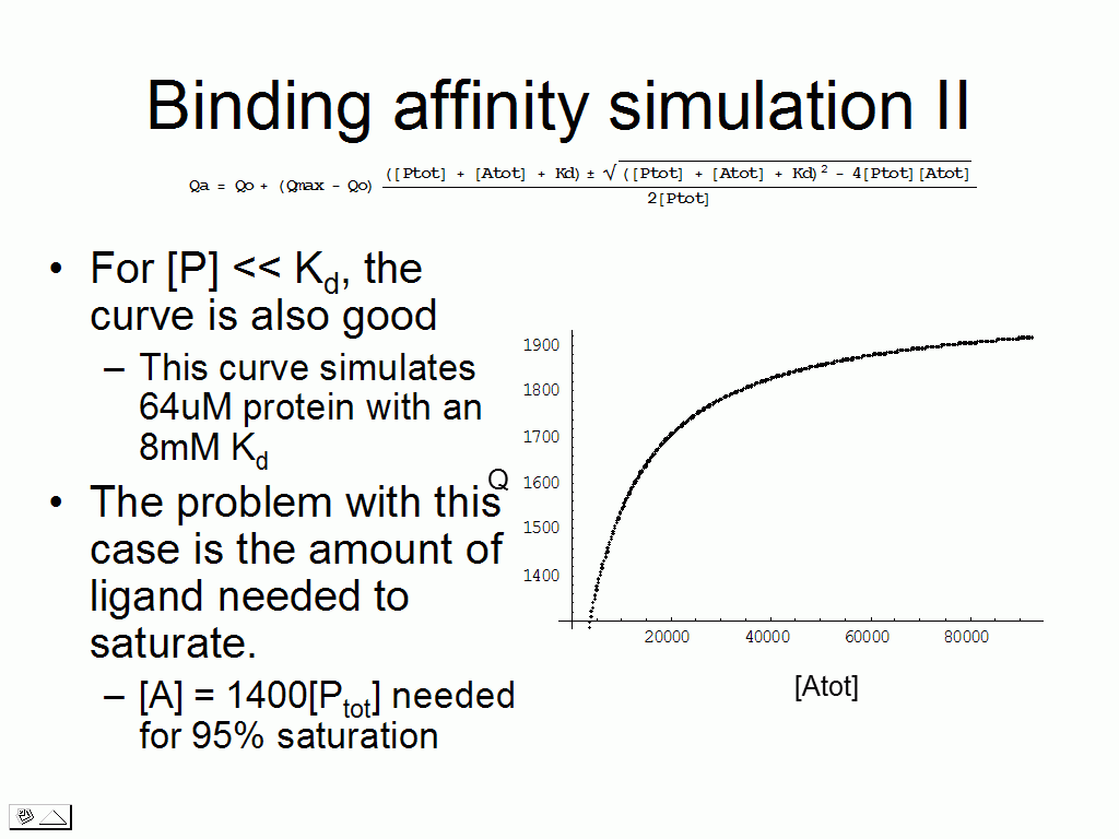
Immediately below is an important but simple equation that represents our assumption that the response being measured (Q) varies linearly with the proportion of protein in the bound state as compared to total protein present. Combining this equation with our results from the quadratic equation above yields the final equation.

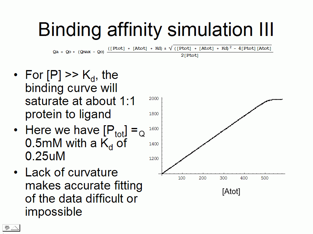
We can test various scenarios to realize that for certain combinations of Kd and protein concentration, there are issues to making the measurement (requires a vast excess of ligand, the binding plot is linear).

Below I provide a Mathematica program for running these simulations. 

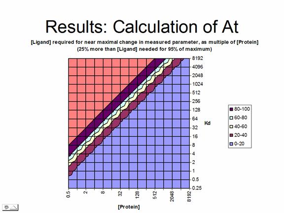
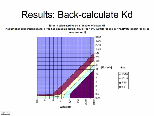
The overall results of the calculation testing a wide range of Kd/protein concentration combinations is that protein in excess of 10-50*Kd results in very large errors in measurement, whereas small amounts of protein with weak binding require a large excess of ligand to achieve saturation.  These results are summed up in the two graphs beow.

Instructions on using the Mathematica program for Kd simulation:

To get the Mathematica notebook, right click the above link and "Save Target As" to a folder. The notebook was written and tested in Mathematica 4.0.

Enter the parameters.  The first two parameters are self descriptive.   The program assumes that the units used for [Protein] and Kd are IDENTICAL.  Therefore if you estimate ~10uM Kd but have 0.5mM protein, adjust one of the numbers so that the units match. 

'EstimatedPercentSaturation' tells the program how far out it should go in the simulation.  Do NOT enter values at above 100,  the program will run forever.

'PercentGaussianError' tells the program how much error to introduce at each data point.  The percent given by here will represent 1 standard deviation in a Gaussian distribution around the value of the data point.  While this leads to a violation of one of the fundamental assumptions

of nonlinear regression, the effect is minor.

'IterationsForErrorEvaluation' controls the number of times that the program should run with the combination of parameters you've entered.   On each iteration, the program compares the back -calculated Kd to the actual starting Kd to achieve an absolute value error estimate.

Once you've entered your parameters, press [SHIFT] - [ENTER] to run the program. 

Output consists of a representative plot of the simulated binding titration with and without Gaussian error introduced.  Three numbers follow:

 the first is the error in Kd calculated over the number of iterations specified,

 while the second and third are the overall average values obtained for fitting Qo and Qmax.

 This is followed by a representative set of fitting diagnostics from a single iteration of the nonlinear fit.  This includes standard error,  confidence intervals, etc.  The final number displayed is the number of times the calculation

failed.